Contents
- Strategy
- Data Preparation
- Useful Methods
- Logistic Model
- Random Decision Forest Classifier (Unlimited Depth) Model
- Random Decision Forest Classifier (Depth-Limited) Model
- K Nearest Neighbors (kNN) Model
- Neural Network Model
- Model Comparison and Analysis
/Users/MikeBao/anaconda3/envs/py36/lib/python3.6/site-packages/sklearn/ensemble/weight_boosting.py:29: DeprecationWarning: numpy.core.umath_tests is an internal NumPy module and should not be imported. It will be removed in a future NumPy release.
  from numpy.core.umath_tests import inner1d
Strategy
As return-maximizing investors in Lending Club (statistical parity to come later), we are concerned with maximizing the expected annual interest rate we can collect by lending capital to borrowers through lending club. Interest rates are exogenous to us and set by LC; hence, our job is to determine the true credit-worthiness of a borrower, taking interest rate as a given. Our models seek to determine $\text{P} \in [0,1]$ in the following expression:
We use the 2016 Q1 LC database to train and test our models. We have discarded all observations that do not belong to the following classifiers: Fully Paid ${1}$ and Charged Off ${0}$ (see EDA for more information). In this form, we can express the problem of loan selection as a binary classification problem. Because all of the models performed herein can express their predictions as probabilities, we are able to determine P for every loan in the test set.
After we have optimized our models to determine P, we will multiply the predicted estimate of P for each loan by its interest rate. This is equal to $\text{E}[\text{Interest Rate}]$. We sort these from largest to smallest. The top n in this list are the best_loans, and they can be averaged to determine the average interest rate of our investment strategy.
Data Preparation
Separate Dependent and Independent Predictors
We begin by looking at the training data and preparing the data for input into our models. These steps largely consist of removing columns that are not known to Lending Club investors when selecting applicants to loan, such as whether or not the loan was fully paid or charged off.
df = pd.read_csv('training_data_v1.csv', skiprows=0)
df_1 = df.copy()
df_1 = df_1.drop(['predictor','Charged Off','Y','N', 'funded_amnt'],axis=1)
df_1['zip_code'] = df['zip_code'].astype(str)
df_new = pd.DataFrame()
df_new = pd.get_dummies(df_1['zip_code'])
df_1 = df_1.drop(['zip_code'],axis=1)
df_1 = pd.concat([df_1,df_new], axis=1)
Impute Missing Data
Since we now have many columns of predictors, we want to determine which columns in our dataset will be the most significant predictors so that we can run our models on a reasonable subset of these predictors. We use a Random Forest Regressor to perform this analysis. Before we do so, we work with a smaller sample of the data and impute missing data. We go through the columns with missing data and decide that imputing 0 is a reasonable step, since many of these columns are of integer type and have low, positive values. For example, a column with missing data was number of delinquicies, with the median number being 0.
Once we have the columns that are the most significant predictors, we will use these columns as input into our models.
sample = df_1.sample(frac=0.01)
for i in sample.index:
    for j in sample.columns:
        if pd.isnull(df_1.at[i,j]):
            sample.at[i,j] = 0
x_train, x_test, y_train, y_test = train_test_split(sample.drop(['Fully Paid'],axis=1),
                                                    sample['Fully Paid'], test_size=0.15, random_state=42)
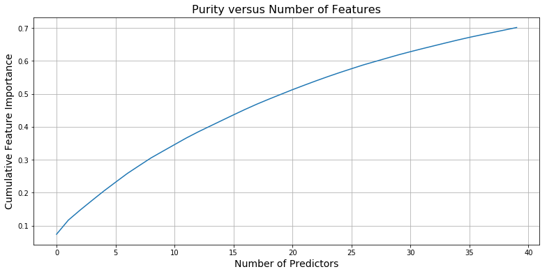
Select Most Significant Predictors Using Random Forest Regressor
In order to make our model building process both feasible and streamlined, we first choose the most significant predictors that we wish to train on. Using a Random Decision Forest Regressor model that we fit on the entire dataset with all of the features, we were able to determine which features contributed the most to increasing the purity of our model. From these features, we selected the 120 predictors that best reflected the datset through increasing purity of estimates and isolated these predictors in a separate dataframe, effectively simulating a forward selection methodology for limiting the predictor space. We used this dataframe to train our models.
rf = RandomForestRegressor()
rf.fit(x_train, y_train)

names = x_train.columns
performance = sorted(zip(map(lambda x: round(x, 4), rf.feature_importances_), names),
             reverse=True)

purity = 0
purity_list = []
selected_cols = []

for i in range(0,40):
    purity = purity + performance[i][0]
    purity_list.append(purity)
    selected_cols.append(performance[i][1])

selected_cols.append('Fully Paid')
plt.figure(figsize=(13, 6))
plt.grid(True)
plt.plot(purity_list);
plt.xlabel("Number of Predictors", size=14);
plt.ylabel("Cumulative Feature Importance", size=14);
plt.title("Purity versus Number of Features", size=16);
print(selected_cols)
['sub_grade', 'mths_since_rcnt_il', 'dti', 'tot_hi_cred_lim', 'all_util', 'avg_cur_bal', 'int_rate', 'total_rev_hi_lim', 'pct_tl_nvr_dlq', 'max_bal_bc', 'installment', 'revol_util', 'num_bc_tl', 'total_acc', 'total_bc_limit', 'bc_util', 'num_rev_accts', 'num_il_tl', 'bc_open_to_buy', 'annual_inc', 'mort_acc', ' 36 months', 'open_rv_12m', 'percent_bc_gt_75', 'tot_cur_bal', 'total_bal_il', 'il_util', 'num_bc_sats', 'acc_open_past_24mths', '103', 'inq_last_12m', 'total_il_high_credit_limit', 'PA', '1 year', 'revol_bal', 'inq_fi', 'open_acc', 'total_cu_tl', 'total_bal_ex_mort', 'num_actv_bc_tl', 'Fully Paid']
df_2 = df_1[selected_cols]
sample2 = df_2.sample(frac=0.1)
for i in sample2.index:
    for j in sample2.columns:
        if pd.isnull(df_1.at[i,j]):
            sample2.at[i,j] = 0
x_train2, x_test2, y_train2, y_test2 = train_test_split(sample2.drop(['Fully Paid'],axis=1),
                                                    sample2['Fully Paid'], test_size=0.15, random_state=42)
Useful Methods
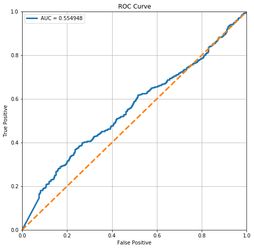
def plot_roc(model):
    roc = roc_curve(y_test2, model.predict_proba(x_test2)[:,1])
    fig, ax = plt.subplots(1,1,figsize=(8,8))
    ax.set_ylim(0,1)
    ax.set_xlim(0,1)
    ax.plot(roc[0],roc[1], linewidth=3)
    ax.set_xlabel('False Positive')
    ax.set_ylabel('True Positive')
    ax.set_title('ROC Curve')
    ax.plot([0,1],[0,1], '--', linewidth=3)
    area = auc(roc[0], roc[1])
    ax.legend(['AUC = %f' % (area)])
    ax.grid(True)
    return area
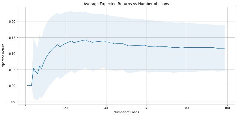
def plot_int(expected_interest):
    ave_rates = []
    std_rates = []
    for i in range(100):
        actual_interest = []
        exp_int_df = pd.DataFrame(data = expected_interest, columns=['EI'])
        best_ten_loans = exp_int_df.sort_values('EI',ascending=False).index[0:i]
        for i in best_ten_loans:
            actual_interest.append(y_test2.iloc[i] * x_test2.iloc[i]['int_rate'])
        ave_rates.append(np.mean(actual_interest))
        std_rates.append(np.std(actual_interest))
    plt.figure(figsize=(13, 6))
    plt.grid(True)
    plt.plot(range(100), ave_rates)
    plt.title('Average Expected Returns vs Number of Loans')
    plt.xlabel('Number of Loans')
    plt.ylabel('Expected Return')
    plt.fill_between(range(100), np.subtract(ave_rates, std_rates), np.add(ave_rates, std_rates), alpha=0.1)
def get_demographic_data(list_of_indices, lending_data, race_data, prop_=['White Proportion','Black Proportion','Asian Proportion','Other Proportion',
                                                                          'Hispanic Proportion','Non-Hispanic Proportion']):

    average_proportions = {}

    for race in prop_:

        race_proportion = []
        for i in list_of_indices:

            zipCode = lending_data.loc[i]['zip_code']

            # accounting for the fact that Lending Club let users input Zip Codes that don't exist in the USA
            try:
                proportion = ((race_data.loc[race_data['Zip Code'] == zipCode][race]).values)
                race_proportion.append(float(proportion))
            except:
                continue


        average_proportions[race] = sum(race_proportion)/len(race_proportion)

    return average_proportions
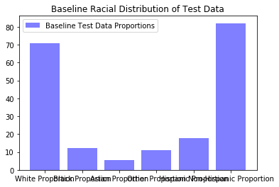
racial_data = pd.read_csv('Race_by_zip_final.csv')

baseline_data_proportions=get_demographic_data(x_test2.index,df,racial_data)
plt.bar(range(len(baseline_data_proportions)), list(baseline_data_proportions.values()), align='center',alpha=0.5,color='blue')
plt.xticks(range(len(baseline_data_proportions)), list(baseline_data_proportions.keys()));
plt.legend(['Baseline Test Data Proportions'])
plt.title("Baseline Racial Distribution of Test Data");
Logistic Model
We now build a logistic regression model that, given input data about loan applications, outputs a number that represents the probability that a specific loan application will be fully paid. We see that our model outputs a score of 0.75.
Instantiate and Fit Logistic Model
x_train2, x_test2, y_train2, y_test2 = train_test_split(sample2.drop(['Fully Paid'],axis=1),
                                                    sample2['Fully Paid'], test_size=0.15, random_state=42)
logistic = LogisticRegressionCV(Cs=1000,penalty='l2')
logistic.fit(x_train2, y_train2)
LogisticRegressionCV(Cs=1000, class_weight=None, cv=None, dual=False,
           fit_intercept=True, intercept_scaling=1.0, max_iter=100,
           multi_class='ovr', n_jobs=1, penalty='l2', random_state=None,
           refit=True, scoring=None, solver='lbfgs', tol=0.0001, verbose=0)
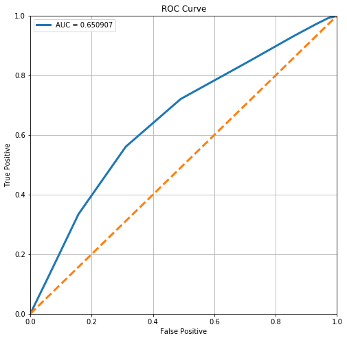
stats.loc['Logistic', 'ROC AUC'] = plot_roc(logistic)
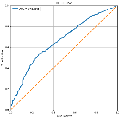
From the ROC Curve, we can see that there is a moderate tradeoff between this model’s sensitivity and its specificity. However, it is still somewhat off from the perfect ROC curve. The perfect ROC has a AUC of 1 (area under curve).
logistic.score(x_test2, y_test2)
stats.loc['Logistic', 'Test Accuracy'] = logistic.score(x_test2, y_test2)
Evaluate Average Interest Returns
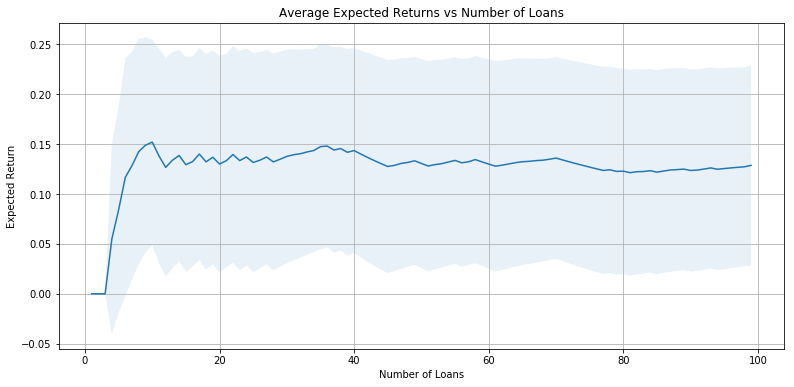
Now that we have a probability for each application, we will calculate our average interest rate returns. For each loan application, we multiply the interest rate assigned by Lending Club by our predicted probability that the loan is fully paid off. This represents the expected interest rate return from a specific loan.
Our investment strategy, then, is to pick the top 10% of loans based off of the expected interest rate return. Based off of this strategy, we see that we expect around 11.2% returns.
original_indices = list(x_test2.index)
expected_interest = []
predicted_prob = logistic.predict_proba(x_test2)
for i in range(0,len(x_test2)):
    # Expected interest is predicted probability times interest rate
    expected_interest.append(predicted_prob[i][1]*x_test2.iloc[i]['int_rate'])
exp_int_df = pd.DataFrame(
    {'original_index': original_indices,
     'EI': expected_interest
    })
top_10_percent = round(len(x_test2)*.1)
best_ten_loans = exp_int_df.sort_values('EI',ascending=False)[0:top_10_percent]
successes = []
for i in best_ten_loans.index:
    successes.append(y_test2.iloc[i])
actual_interest = []
for i in best_ten_loans.index:
    actual_interest.append(x_test2.iloc[i]['int_rate']*y_test2.iloc[i])
stats.loc['Logistic', 'Investment Returns'] = np.mean(actual_interest)
np.mean(actual_interest)
0.12606557377049177
plot_int(expected_interest)
expected_interests.append(expected_interest)
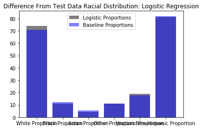
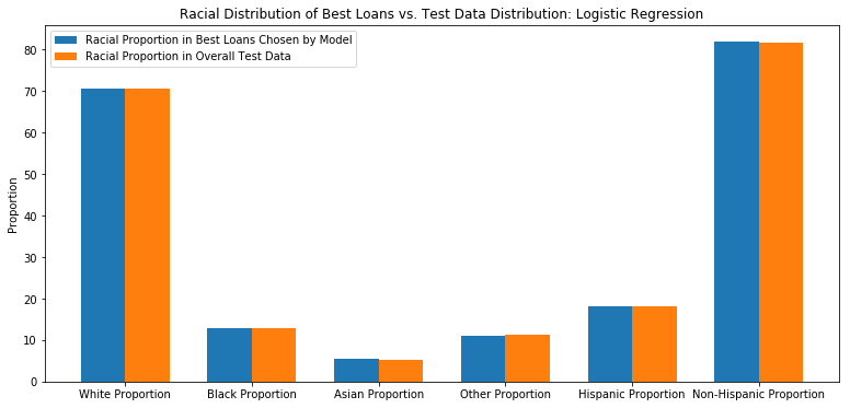
Evaluate Racial Distribution of Best Loans
Having already determined the top 10% of loans by their individual expected interet rates (i.e. percentage return), we will now determine the expected racial distribution of this bag of loans. Using the racial distributions of the populations underlying the three-digit zip codes provided by Lending Club, we can determine the aveerage percentage of each racial group represented in this bag of loans.
racial_percentage_logistic = {}
racial_percentage_logistic = get_demographic_data(best_ten_loans['original_index'],df,racial_data)
plt.bar(range(len(racial_percentage_logistic)), list(racial_percentage_logistic.values()), align='center',alpha=0.5,color='black')
plt.bar(range(len(baseline_data_proportions)), list(baseline_data_proportions.values()), align='center',alpha=0.5,color='blue')
plt.xticks(range(len(racial_percentage_logistic)), list(racial_percentage_logistic.keys()));
plt.legend(['Logistic Proportions','Baseline Proportions'])
plt.title("Difference From Test Data Racial Distribution: Logistic Regression");
Random Decision Forest Classifier (Unlimited Depth) Model
Build and Instantiate Random Decision Forest Classifier Model
We run a random forest classifier and determining which depth gives the best test accuracy. We then select this depth moving forward, using the probabilities calculated using this depth to calculate our average expected returns. We achieve an expected return of about 11.6%.
forest = RandomForestClassifier().fit(x_train2, y_train2)
stats.loc['Decision Forest (Unlimited)', 'Test Accuracy'] = forest.score(x_test2, y_test2)
forest.score(x_test2, y_test2)
0.7001633986928104
stats.loc['Decision Forest (Unlimited)', 'ROC AUC'] = plot_roc(forest)
From the ROC Curve, we can see that there is a moderate tradeoff between this model’s sensitivity and its specificity. However, it is still somewhat off from the perfect ROC curve. The perfect ROC curve would have an area under curve of 1.
prob_array = forest.predict_proba(x_test2)
Evaulate Average Interest Returns
original_indices = list(x_test2.index)
expected_interest = []
for i in range(0,len(x_test2)):
    expected_interest.append(forest.predict(x_test2)[i] * prob_array[i][1]*x_test2.iloc[i]['int_rate'])
exp_int_df = pd.DataFrame(
    {'original_index': original_indices,
     'EI': expected_interest
    })
best_ten_loans = exp_int_df.sort_values('EI',ascending=False)[0:int(len(x_test2)*0.1)]
actual_interest = []
for i in best_ten_loans.index:
    actual_interest.append(y_test2.iloc[i] * x_test2.iloc[i]['int_rate'])
stats.loc['Decision Forest (Unlimited)', 'Investment Returns'] = np.mean(actual_interest)
np.mean(actual_interest)
0.1268032786885246
plot_int(expected_interest)
expected_interests.append(expected_interest)
Evaluate Racial Distribution of Best Loans
racial_percentage_tree = {}
racial_percentage_tree = get_demographic_data(best_ten_loans['original_index'],df,racial_data)
model_data = list(racial_percentage_logistic.values())
baseline_data = list(baseline_data_proportions.values())

ind = np.arange(len(model_data))
width = 0.35

fig, ax = plt.subplots()
rects1 = ax.bar(ind - width/2, model_data, width, label='Logit')
rects2 = ax.bar(ind + width/2, baseline_data, width, label='Baseline')

ax.set_ylabel('Proportion')
ax.set_title('Racial Distribution of Best Loans vs. Test Data Distribution: Logistic Regression')
ax.set_xticks(ind)
ax.set_xticklabels(list(racial_percentage_logistic.keys()))
ax.legend(["Racial Proportion in Best Loans Chosen by Model","Racial Proportion in Overall Test Data"]);
Tree Structure Analysis
We output the decision tree structure to gain insight into the important features.
def show_tree_structure(clf):
    tree = clf.tree_

    n_nodes = tree.node_count
    children_left = tree.children_left
    children_right = tree.children_right
    feature = tree.feature
    threshold = tree.threshold

    # The tree structure can be traversed to compute various properties such
    # as the depth of each node and whether or not it is a leaf.
    node_depth = np.zeros(shape=n_nodes, dtype=np.int64)
    is_leaves = np.zeros(shape=n_nodes, dtype=bool)
    stack = [(0, -1)]  # seed is the root node id and its parent depth
    while len(stack) > 0:
        node_id, parent_depth = stack.pop()
        node_depth[node_id] = parent_depth + 1

        # If we have a test node
        if (children_left[node_id] != children_right[node_id]):
            stack.append((children_left[node_id], parent_depth + 1))
            stack.append((children_right[node_id], parent_depth + 1))
        else:
            is_leaves[node_id] = True

    print(f"The binary tree structure has {n_nodes} nodes:\n")
    i = 0
    for i in range(n_nodes):
        indent = node_depth[i] * "  "
        if is_leaves[i]:
            prediction = clf.classes_[np.argmax(tree.value[i])]
            print(f"{indent}node {i}: predict class {prediction}")
        else:
            print("{}node {}: if X[:, {}] <= {:.3f} then go to node {}, else go to node {}".format(
                indent, i, x_train2.columns[feature[i]], threshold[i], children_left[i], children_right[i]))
        i += 1
        if i > 50:
            break
show_tree_structure(forest.estimators_[0])
The binary tree structure has 1941 nodes:

node 0: if X[:, mths_since_rcnt_il] <= 4.500 then go to node 1, else go to node 438
  node 1: if X[:, sub_grade] <= 11.500 then go to node 2, else go to node 163
    node 2: if X[:, revol_bal] <= 10002.500 then go to node 3, else go to node 74
      node 3: if X[:, revol_util] <= 0.945 then go to node 4, else go to node 71
        node 4: if X[:, avg_cur_bal] <= 14237.500 then go to node 5, else go to node 64
          node 5: if X[:, avg_cur_bal] <= 13816.500 then go to node 6, else go to node 63
            node 6: if X[:, dti] <= 27.870 then go to node 7, else go to node 58
              node 7: if X[:, total_bal_ex_mort] <= 847.500 then go to node 8, else go to node 9
                node 8: predict class 0.0
                node 9: if X[:, inq_fi] <= 5.500 then go to node 10, else go to node 55
                  node 10: if X[:, bc_open_to_buy] <= 2605.000 then go to node 11, else go to node 18
                    node 11: if X[:, num_il_tl] <= 8.500 then go to node 12, else go to node 13
                      node 12: predict class 1.0
                      node 13: if X[:, open_rv_12m] <= 1.500 then go to node 14, else go to node 15
                        node 14: predict class 1.0
                        node 15: if X[:, inq_fi] <= 1.000 then go to node 16, else go to node 17
                          node 16: predict class 0.0
                          node 17: predict class 1.0
                    node 18: if X[:, total_rev_hi_lim] <= 6850.000 then go to node 19, else go to node 20
                      node 19: predict class 0.0
                      node 20: if X[:, sub_grade] <= 6.500 then go to node 21, else go to node 30
                        node 21: if X[:, percent_bc_gt_75] <= 16.250 then go to node 22, else go to node 27
                          node 22: if X[:, max_bal_bc] <= 301.500 then go to node 23, else go to node 26
                            node 23: if X[:, num_actv_bc_tl] <= 1.500 then go to node 24, else go to node 25
                              node 24: predict class 1.0
                              node 25: predict class 0.0
                            node 26: predict class 1.0
                          node 27: if X[:, revol_bal] <= 6159.000 then go to node 28, else go to node 29
                            node 28: predict class 1.0
                            node 29: predict class 0.0
                        node 30: if X[:, tot_hi_cred_lim] <= 14086.000 then go to node 31, else go to node 34
                          node 31: if X[:, revol_bal] <= 2885.500 then go to node 32, else go to node 33
                            node 32: predict class 1.0
                            node 33: predict class 0.0
                          node 34: if X[:, annual_inc] <= 75500.000 then go to node 35, else go to node 54
                            node 35: if X[:, percent_bc_gt_75] <= 41.650 then go to node 36, else go to node 51
                              node 36: if X[:, annual_inc] <= 71000.000 then go to node 37, else go to node 48
                                node 37: if X[:, total_bal_il] <= 7991.500 then go to node 38, else go to node 43
                                  node 38: if X[:, total_acc] <= 26.000 then go to node 39, else go to node 42
                                    node 39: if X[:, tot_hi_cred_lim] <= 43250.000 then go to node 40, else go to node 41
                                      node 40: predict class 1.0
                                      node 41: predict class 0.0
                                    node 42: predict class 0.0
                                  node 43: if X[:, total_cu_tl] <= 6.500 then go to node 44, else go to node 45
                                    node 44: predict class 1.0
                                    node 45: if X[:, num_il_tl] <= 11.000 then go to node 46, else go to node 47
                                      node 46: predict class 0.0
                                      node 47: predict class 1.0
                                node 48: if X[:, total_cu_tl] <= 4.000 then go to node 49, else go to node 50
                                  node 49: predict class 0.0
                                  node 50: predict class 1.0
Random Decision Forest Classifier (Depth-Limited) Model
Build and Instantiate Random Decision Forest Classifier Model
We run a random forest classifier and determining which depth gives the best test accuracy. We then select this depth moving forward, using the probabilities calculated using this depth to calculate our average expected returns. We achieve an expected return of about 11.6%.
test_scores = []
cross_val_scores = []
cross_val_stdevs = []
forests = []
d = 18
plt.figure(figsize=(12,7))
for depth in range(2,d):
    forest = RandomForestClassifier(max_depth=depth)
    forest.fit(x_train2, y_train2)
    test_scores.append(forest.score(x_test2, y_test2))
    cross_val = cross_val_score(forest, x_train2, y_train2, cv=5)
    cross_val_scores.append(sum(cross_val)/5.0)
    cross_val_stdevs.append(math.sqrt(np.var(np.asarray(cross_val))))
    forests.append(forest)
plt.plot(range(2,d), cross_val_scores)
plt.plot(range(2,d), test_scores)
plt.fill_between(range(2,d),
                 [x - y  for x,y in zip(cross_val_scores, cross_val_stdevs)],
                 [x + y  for x,y in zip(cross_val_scores, cross_val_stdevs)],
                alpha = 0.3)
plt.xlabel('Max Depth', size=14)
plt.ylabel('Score', size=14)
plt.grid(True)
plt.title('Scores of Random Forest Classifier')
plt.legend(['Cross Validation Scores', 'Test Accuracies']);
plt.rcParams['figure.figsize'] = (13.0, 6.0);
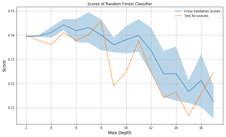
idx = np.argmax(test_scores)
stats.loc['Decision Forest (Limited)', 'Test Accuracy'] = forests[idx].score(x_test2, y_test2)
forests[idx].score(x_test2, y_test2)
0.7459150326797386
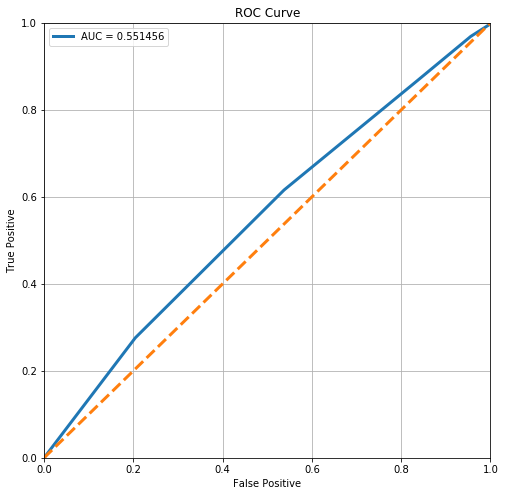
stats.loc['Decision Forest (Limited)', 'ROC AUC'] = plot_roc(forests[idx])
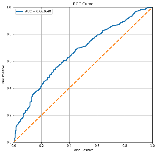
From the ROC Curve, we can see that there is a relatively lower tradeoff between this model’s sensitivity and its specificity. However, it is still somewhat off from the perfect ROC curve.
prob_array = forests[idx].predict_proba(x_test2)
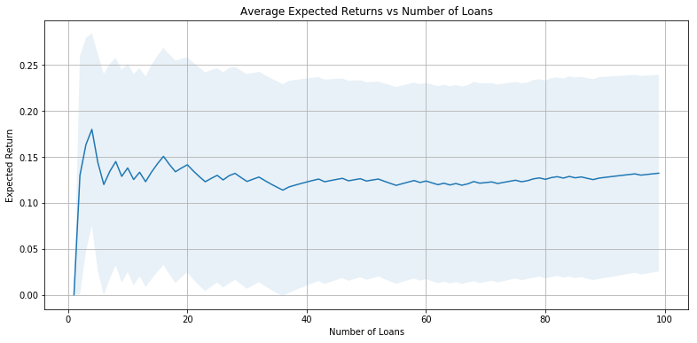
Evaulate Average Interest Returns
original_indices = list(x_test2.index)
expected_interest = []
for i in range(0,len(x_test2)):
    expected_interest.append(forests[idx].predict(x_test2)[i] * prob_array[i][1]*x_test2.iloc[i]['int_rate'])
exp_int_df = pd.DataFrame(
    {'original_index': original_indices,
     'EI': expected_interest
    })
best_ten_loans = exp_int_df.sort_values('EI',ascending=False)[0:int(len(x_test2)*0.1)]
actual_interest = []
for i in best_ten_loans.index:
    actual_interest.append(y_test2.iloc[i] * x_test2.iloc[i]['int_rate'])
stats.loc['Decision Forest (Limited)', 'Investment Returns'] = np.mean(actual_interest)
np.mean(actual_interest)
0.11901639344262294
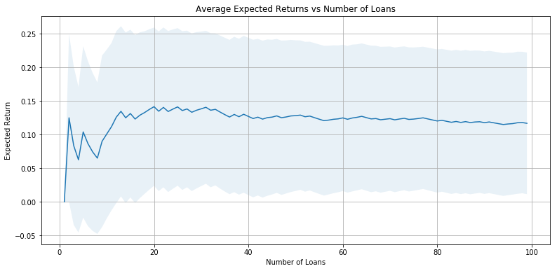
plot_int(expected_interest)
expected_interests.append(expected_interest)
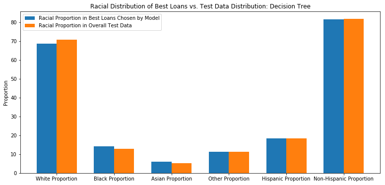
Evaluate Racial Distribution of Best Loans
racial_percentage_rf = {}
racial_percentage_rf = get_demographic_data(best_ten_loans['original_index'],df,racial_data)
racial_percentage_rf
{'White Proportion': 70.1413569702473,
 'Black Proportion': 13.882252044573503,
 'Asian Proportion': 4.583658222145505,
 'Other Proportion': 11.396783756100392,
 'Hispanic Proportion': 19.41150341363492,
 'Non-Hispanic Proportion': 80.58836532899765}
model_data = list(racial_percentage_tree.values())
baseline_data = list(baseline_data_proportions.values())

ind = np.arange(len(model_data))
width = 0.35

fig, ax = plt.subplots()
rects1 = ax.bar(ind - width/2, model_data, width, label='Decision Tree')
rects2 = ax.bar(ind + width/2, baseline_data, width, label='Baseline')

ax.set_ylabel('Proportion')
ax.set_title('Racial Distribution of Best Loans vs. Test Data Distribution: Decision Tree')
ax.set_xticks(ind)
ax.set_xticklabels(list(racial_percentage_tree.keys()))
ax.legend(["Racial Proportion in Best Loans Chosen by Model","Racial Proportion in Overall Test Data"]);
We output the decision tree structure to gain insight into the important features.
Tree Structure Analysis
def show_tree_structure(clf):
    tree = clf.tree_

    n_nodes = tree.node_count
    children_left = tree.children_left
    children_right = tree.children_right
    feature = tree.feature
    threshold = tree.threshold

    # The tree structure can be traversed to compute various properties such
    # as the depth of each node and whether or not it is a leaf.
    node_depth = np.zeros(shape=n_nodes, dtype=np.int64)
    is_leaves = np.zeros(shape=n_nodes, dtype=bool)
    stack = [(0, -1)]  # seed is the root node id and its parent depth
    while len(stack) > 0:
        node_id, parent_depth = stack.pop()
        node_depth[node_id] = parent_depth + 1

        # If we have a test node
        if (children_left[node_id] != children_right[node_id]):
            stack.append((children_left[node_id], parent_depth + 1))
            stack.append((children_right[node_id], parent_depth + 1))
        else:
            is_leaves[node_id] = True

    print(f"The binary tree structure has {n_nodes} nodes:\n")
    i = 0
    for i in range(n_nodes):
        indent = node_depth[i] * "  "
        if is_leaves[i]:
            prediction = clf.classes_[np.argmax(tree.value[i])]
            print(f"{indent}node {i}: predict class {prediction}")
        else:
            print("{}node {}: if X[:, {}] <= {:.3f} then go to node {}, else go to node {}".format(
                indent, i, x_train2.columns[feature[i]], threshold[i], children_left[i], children_right[i]))
        i += 1
        if i > 50:
            break
show_tree_structure(forests[idx].estimators_[0])
The binary tree structure has 333 nodes:

node 0: if X[:, percent_bc_gt_75] <= 36.050 then go to node 1, else go to node 176
  node 1: if X[:, mort_acc] <= 2.500 then go to node 2, else go to node 89
    node 2: if X[:, int_rate] <= 0.125 then go to node 3, else go to node 52
      node 3: if X[:, num_actv_bc_tl] <= 1.500 then go to node 4, else go to node 27
        node 4: if X[:, total_il_high_credit_limit] <= 4250.000 then go to node 5, else go to node 14
          node 5: if X[:, acc_open_past_24mths] <= 2.500 then go to node 6, else go to node 9
            node 6: if X[:, total_bal_ex_mort] <= 3876.000 then go to node 7, else go to node 8
              node 7: predict class 1.0
              node 8: predict class 0.0
            node 9: if X[:, total_bc_limit] <= 2650.000 then go to node 10, else go to node 13
              node 10: if X[:, inq_fi] <= 0.500 then go to node 11, else go to node 12
                node 11: predict class 0.0
                node 12: predict class 1.0
              node 13: predict class 1.0
          node 14: if X[:, bc_util] <= 52.000 then go to node 15, else go to node 22
            node 15: if X[:, bc_util] <= 42.650 then go to node 16, else go to node 19
              node 16: if X[:, inq_last_12m] <= 10.000 then go to node 17, else go to node 18
                node 17: predict class 1.0
                node 18: predict class 0.0
              node 19: if X[:, total_cu_tl] <= 2.000 then go to node 20, else go to node 21
                node 20: predict class 1.0
                node 21: predict class 0.0
            node 22: if X[:, max_bal_bc] <= 804.500 then go to node 23, else go to node 24
              node 23: predict class 0.0
              node 24: if X[:, sub_grade] <= 10.500 then go to node 25, else go to node 26
                node 25: predict class 1.0
                node 26: predict class 0.0
        node 27: if X[:, int_rate] <= 0.065 then go to node 28, else go to node 39
          node 28: if X[:, installment] <= 475.820 then go to node 29, else go to node 34
            node 29: if X[:, inq_fi] <= 1.500 then go to node 30, else go to node 31
              node 30: predict class 1.0
              node 31: if X[:, il_util] <= 81.500 then go to node 32, else go to node 33
                node 32: predict class 1.0
                node 33: predict class 1.0
            node 34: if X[:, tot_hi_cred_lim] <= 52505.000 then go to node 35, else go to node 36
              node 35: predict class 0.0
              node 36: if X[:, num_bc_sats] <= 2.500 then go to node 37, else go to node 38
                node 37: predict class 0.0
                node 38: predict class 1.0
          node 39: if X[:, installment] <= 482.430 then go to node 40, else go to node 45
            node 40: if X[:, total_bc_limit] <= 1700.000 then go to node 41, else go to node 42
              node 41: predict class 0.0
              node 42: if X[:, tot_hi_cred_lim] <= 276657.500 then go to node 43, else go to node 44
                node 43: predict class 1.0
                node 44: predict class 1.0
            node 45: if X[:, total_cu_tl] <= 9.500 then go to node 46, else go to node 49
              node 46: if X[:, tot_cur_bal] <= 17031.000 then go to node 47, else go to node 48
                node 47: predict class 0.0
                node 48: predict class 1.0
              node 49: if X[:, tot_cur_bal] <= 255394.000 then go to node 50, else go to node 51
                node 50: predict class 0.0
K Nearest Neighbors (kNN) Model
Build and Instantiate KNN Model
Our next model is to build a neural network using sklearn’s KNN classifier. We want our neural network to similarly output the probability that a loan application will be fully paid off. Using this probability, we will then calculate the average interest rate returns, using the same method as described earlier.
We see that our network achieves a score of around 0.74 on both the training data set and the test data set.
clf = KNeighborsClassifier()
clf.fit(x_train2, y_train2)
KNeighborsClassifier(algorithm='auto', leaf_size=30, metric='minkowski',
           metric_params=None, n_jobs=1, n_neighbors=5, p=2,
           weights='uniform')
clf.score(x_train2, y_train2)
0.780952380952381
stats.loc['kNN', 'ROC AUC'] = plot_roc(clf)
From the ROC Curve, we can see that there is a high tradeoff between this model’s sensitivity and its specificity. However, it is still relatively off from the perfect ROC curve, as can be seen by the low AUC score.
stats.loc['kNN', 'Test Accuracy'] = clf.score(x_test2, y_test2)
clf.score(x_test2, y_test2)
0.684640522875817
Evaluate Average Interest Returns
Using our neural network model, we see that we achieve an expected average interest rate return of about 9.53%.
original_indices = list(x_test2.index)
expected_interest = []
for i in range(0,len(x_test2)):
    expected_interest.append(clf.predict_proba(x_test2)[i][1]*x_test2.iloc[i]['int_rate'])
exp_int_df = pd.DataFrame(
    {'original_index': original_indices,
     'EI': expected_interest
    })
best_ten_loans = exp_int_df.sort_values('EI',ascending=False)[0:int(len(x_test2)*0.1)]
successes = []
for i in best_ten_loans.index:
    successes.append(y_test2.iloc[i])
actual_interest = []
for i in best_ten_loans.index:
    actual_interest.append(y_test2.iloc[i] * x_test2.iloc[i]['int_rate'])
stats.loc['kNN', 'Investment Returns'] = np.mean(actual_interest)
np.mean(actual_interest)
0.13352459016393442
plot_int(expected_interest)
expected_interests.append(expected_interest)
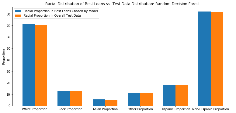
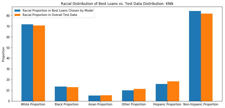
Evaluate Racial Distribution of Best Loans
racial_percentage_knn = {}
racial_percentage_knn = get_demographic_data(best_ten_loans['original_index'],df,racial_data)
racial_percentage_knn
{'White Proportion': 72.2432036501075,
 'Black Proportion': 11.799882010858726,
 'Asian Proportion': 4.507256606145926,
 'Other Proportion': 11.455481974403002,
 'Hispanic Proportion': 20.203251964521886,
 'Non-Hispanic Proportion': 79.79659964546002}
model_data = list(racial_percentage_rf.values())
baseline_data = list(baseline_data_proportions.values())

ind = np.arange(len(model_data))
width = 0.35

fig, ax = plt.subplots()
rects1 = ax.bar(ind - width/2, model_data, width, label='Random Decision Forest')
rects2 = ax.bar(ind + width/2, baseline_data, width, label='Baseline')

ax.set_ylabel('Proportion')
ax.set_title('Racial Distribution of Best Loans vs. Test Data Distribution: Random Decision Forest')
ax.set_xticks(ind)
ax.set_xticklabels(list(racial_percentage_rf.keys()))
ax.legend(["Racial Proportion in Best Loans Chosen by Model","Racial Proportion in Overall Test Data"]);
Neural Network Model
Build and Instantiate Neural Network Model
Our next model is to build a neural network using sklearn’s Multi-layer Perceptron classifier. We want our neural network to similarly output the probability that a loan application will be fully paid off. Using this probability, we will then calculate the average interest rate returns, using the same method as described earlier.
We see that our network achieves a score of around 0.74 on both the training data set and the test data set.
clf = MLPClassifier(solver='adam', alpha=1e-1, hidden_layer_sizes=(160,80,40,20), random_state=1, max_iter=10000)
clf.fit(x_train2, y_train2)
MLPClassifier(activation='relu', alpha=0.1, batch_size='auto', beta_1=0.9,
       beta_2=0.999, early_stopping=False, epsilon=1e-08,
       hidden_layer_sizes=(160, 80, 40, 20), learning_rate='constant',
       learning_rate_init=0.001, max_iter=10000, momentum=0.9,
       nesterovs_momentum=True, power_t=0.5, random_state=1, shuffle=True,
       solver='adam', tol=0.0001, validation_fraction=0.1, verbose=False,
       warm_start=False)
clf.score(x_train2, y_train2)
0.43463203463203465
np.mean(clf.predict(x_test2))
0.25163398692810457
stats.loc['Neural Network', 'ROC AUC'] = plot_roc(clf)
From the ROC Curve, we can see that there is a high tradeoff between this model’s sensitivity and its specificity. However, it is relatively far off from the perfect ROC curve, since the AUC is relatively low.
stats.loc['Neural Network', 'Test Accuracy'] = clf.score(x_test2, y_test2)
clf.score(x_test2, y_test2)
0.42483660130718953
Evaluate Average Interest Returns
Using our neural network model, we see that we achieve an expected average interest rate return of about 9.53%.
original_indices = list(x_test2.index)
expected_interest = []
for i in range(0,len(x_test2)):
    expected_interest.append(clf.predict_proba(x_test2)[i][1]*x_test2.iloc[i]['int_rate'])
exp_int_df = pd.DataFrame(
    {'original_index': original_indices,
     'EI': expected_interest
    })
best_ten_loans = exp_int_df.sort_values('EI',ascending=False)[0:int(len(x_test2)*0.1)]
successes = []
for i in best_ten_loans.index:
    successes.append(y_test2.iloc[i])
actual_interest = []
for i in best_ten_loans.index:
    actual_interest.append(y_test2.iloc[i] * x_test2.iloc[i]['int_rate'])
stats.loc['Neural Network', 'Investment Returns'] = np.mean(actual_interest)
np.mean(actual_interest)
0.11295081967213115
plot_int(expected_interest)
expected_interests.append(expected_interest)
Evaluate Racial Distribution of Best Loans
racial_percentage_nn = {}
racial_percentage_nn = get_demographic_data(best_ten_loans['original_index'],df,racial_data)
racial_percentage_nn
{'White Proportion': 69.68824817410244,
 'Black Proportion': 13.50434161259944,
 'Asian Proportion': 5.66088724446923,
 'Other Proportion': 11.15064225866612,
 'Hispanic Proportion': 19.513095962841458,
 'Non-Hispanic Proportion': 80.48677554615921}
model_data = list(racial_percentage_knn.values())
baseline_data = list(baseline_data_proportions.values())

ind = np.arange(len(model_data))
width = 0.35

fig, ax = plt.subplots()
rects1 = ax.bar(ind - width/2, model_data, width, label='KNN')
rects2 = ax.bar(ind + width/2, baseline_data, width, label='Baseline')

ax.set_ylabel('Proportion')
ax.set_title('Racial Distribution of Best Loans vs. Test Data Distribution: KNN')
ax.set_xticks(ind)
ax.set_xticklabels(list(racial_percentage_knn.keys()))
ax.legend(["Racial Proportion in Best Loans Chosen by Model","Racial Proportion in Overall Test Data"]);
Model Comparison and Analysis
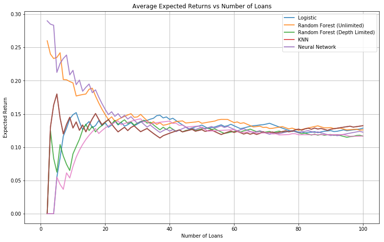
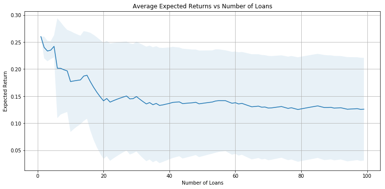
Expected Returns Analysis
plt.figure(figsize=(13,8))
for expected_interest in expected_interests:
    ave_rates = []
    std_rates = []
    for i in range(100):
        actual_interest = []
        exp_int_df = pd.DataFrame(data = expected_interest, columns=['EI'])
        best_ten_loans = exp_int_df.sort_values('EI',ascending=False).index[0:i]
        for i in best_ten_loans:
            actual_interest.append(y_test2.iloc[i] * x_test2.iloc[i]['int_rate'])
        ave_rates.append(np.mean(actual_interest))
        std_rates.append(np.std(actual_interest))
    plt.plot(range(101), [0] + ave_rates, lw=2, alpha=0.8)
plt.grid(True)
plt.title('Average Expected Returns vs Number of Loans')
plt.xlabel('Number of Loans')
plt.ylabel('Expected Return')
plt.legend(['Logistic', 'Random Forest (Unlimited)', 'Random Forest (Depth Limited)', 'KNN', 'Neural Network']);